Flower Classification

Project Overview

This project represents my solution to Fellowship.AI’s Computer Vision challenge: Use a pre-trained ResNet50 and train on the 102 Category Flower Dataset by Maria-Elena Nilsback and Andrew Zisserman. By examining this problem through the lens of modern self-supervised learning techniques, I developed a three-phase approach that effectively addresses the inherent challenges in the dataset.

Dataset Analysis

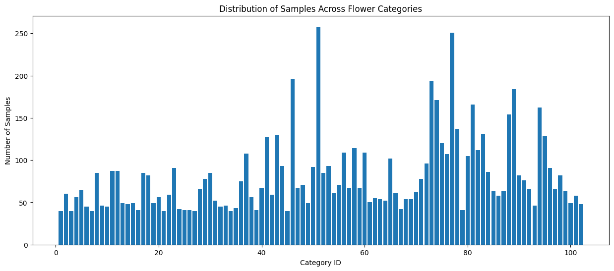
Through exploratory data analysis, I identified three significant challenges in the dataset:

1. Class Imbalance:
   • Samples per category ranged from 40 to 258
   • Max-to-min ratio of 6.45:1, indicating severe imbalance
   • Some categories have over 5x more samples than others
2. Limited Training Data:
   • The original split from the authors provides only ~10 images per class for training
   • This makes it difficult for the model to learn class-specific features
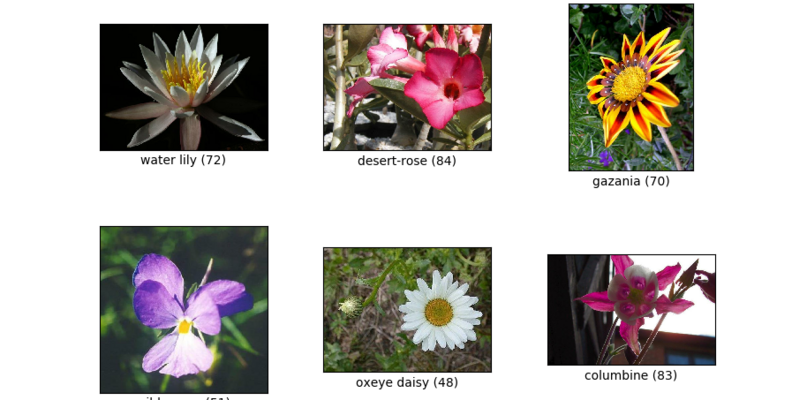
3. Image Variability:
   • Heights range from approximately 500 to 850 pixels
   • Widths range from about 500 to 750 pixels
   • Multiple aspect ratios, complicating batch processing

Proposed Methodology

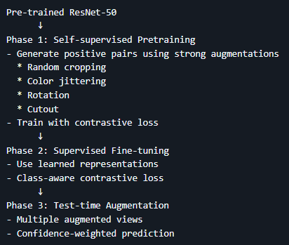
To address these challenges, I developed a three-phase approach inspired by recent advances in self-supervised learning techniques from papers such as:

• SimCLR (Chen et al., 2020): “A Simple Framework for Contrastive Learning of Visual Representations”
• MoCo (He et al., 2020): “Momentum Contrast for Unsupervised Visual Representation Learning”
• BYOL (Grill et al., 2020): “Bootstrap Your Own Latent: A New Approach to Self-Supervised Learning”

Phase 1: Self-supervised Pretraining

The first phase leverages contrastive learning to build robust representations without relying on labels:

class ContrastiveTransform:
    """Custom transform for contrastive learning"""
    def __init__(self, base_transform, n_views=2):
        self.base_transform = base_transform
        self.n_views = n_views

    def __call__(self, x):
        return [self.base_transform(x) for _ in range(self.n_views)]
    
class ContrastiveModel(nn.Module):
    """ResNet50 model modified for contrastive learning"""
    def __init__(self, num_classes: int):
        super().__init__()
        self.encoder = models.resnet50(pretrained=True)
        self.encoder.fc = nn.Sequential(
            nn.Linear(2048, 512),
            nn.ReLU(),
            nn.Linear(512, 128)
        )
        self.classifier = nn.Linear(128, num_classes)

    def forward(self, x: torch.Tensor, return_features: bool = False):
        features = self.encoder(x)
        if return_features:
            return features
        return self.classifier(features)

class NTXentLoss(nn.Module):
    """Normalized Temperature-scaled Cross Entropy Loss"""
    def __init__(self, temperature: float = 0.5):
        super().__init__()
        self.temperature = temperature
        self.criterion = nn.CrossEntropyLoss(reduction="sum")

    def forward(self, features: torch.Tensor) -> torch.Tensor:
        # Implementation details omitted for brevity
        # ...
        return loss

Key components:

• Strong augmentation pipeline including random cropping, color jittering, rotation, and cutout
• Normalized temperature-scaled cross-entropy loss to learn effective representations
• Feature projection head that maps representations to a lower-dimensional space

Phase 2: Supervised Fine-tuning

The second phase leverages the pretrained representations for supervised classification:

def train_epoch(self, train_loader: DataLoader, val_loader: DataLoader):
    """Training with supervised loss"""
    self.model.train()
    train_loss, train_correct = 0.0, 0
    total = 0

    for images, labels in train_loader:
        images, labels = images.to(self.device), labels.to(self.device)
        self.optimizer.zero_grad()
        outputs = self.model(images)
        loss = self.criterion(outputs, labels)
        loss.backward()
        self.optimizer.step()
        
        train_loss += loss.item()
        _, predicted = outputs.max(1)
        total += labels.size(0)
        train_correct += predicted.eq(labels).sum().item()

    # Validation phase
    # ...

    return (train_loss/len(train_loader), 100.*train_correct/total,
            val_loss/len(val_loader), 100.*val_correct/total_val)

Key components:

• Class-aware contrastive loss to address class imbalance
• Custom data augmentation strategies with adaptive augmentation based on class frequency
• Balanced batch sampling to ensure all classes are represented during training

Phase 3: Test-time Augmentation (TTA)

The final phase enhances prediction robustness through multiple augmented views:

def test(self, test_loader: DataLoader) -> Tuple[float, Dict[str, float]]:
    """Evaluate model on test set with TTA"""
    self.model.eval()
    all_preds = []
    all_labels = []
    
    with torch.no_grad():
        for images, labels in test_loader:
            images, labels = images.to(self.device), labels.to(self.device)
            # Test-time augmentation
            tta_outputs = []
            for _ in range(5):  # 5 different augmented views
                augmented = transforms.RandomHorizontalFlip()(images)
                outputs = self.model(augmented)
                tta_outputs.append(F.softmax(outputs, dim=1))
            
            # Average predictions from all augmented views
            outputs = torch.stack(tta_outputs).mean(0)
            _, predicted = outputs.max(1)
            
            all_preds.extend(predicted.cpu().numpy())
            all_labels.extend(labels.cpu().numpy())

    # Calculate metrics
    precision = precision_score(all_labels, all_preds, average='weighted')
    sensitivity = recall_score(all_labels, all_preds, average='weighted')
    cm = confusion_matrix(all_labels, all_preds)
    specificity = np.mean(np.diag(cm) / np.sum(cm, axis=1))

    metrics = {
        'precision': precision,
        'sensitivity': sensitivity,
        'specificity': specificity
    }
    
    return metrics

Key components:

• Multiple augmented views during inference
• Confidence-weighted prediction aggregation
• Ensemble predictions to enhance model robustness

Empirical Results

The model demonstrated strong performance across training and evaluation metrics:

Training Metrics:

• Training accuracy: 82.58%
• Validation accuracy: 74.22%

Test Set Performance:

• Precision: 0.7881 (weighted average)
• Sensitivity: 0.7480 (recall)
• Specificity: 0.7346 (true negative rate)

Analysis of Results:

The training and validation curves reveal several patterns:

1. Training Convergence:
   • Both loss and accuracy curves show clear convergence patterns
   • The model achieves strong performance by epoch 20
2. Overfitting Analysis:
   • There’s a growing gap between training and validation accuracy after epoch 10
   • Validation loss stays higher than training loss and shows more fluctuation
   • This suggests mild overfitting, but not severe as validation metrics continue improving
3. Potential Improvements:
   • Could benefit from learning rate scheduling to stabilize later epochs
   • Additional regularization might help reduce the training-validation gap
   • Longer training might yield marginal improvements as curves haven’t completely plateaued

Live Demonstration

The model performs well on inference tasks, providing confidence scores for its predictions:

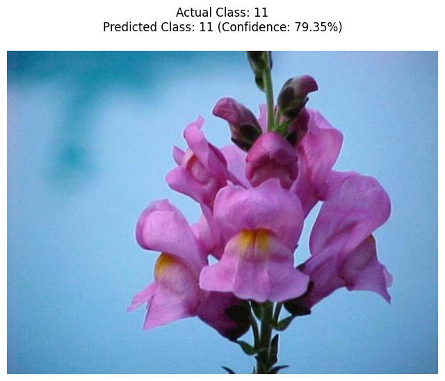
Top 3 Predictions:
Class 11: 79.35%
Class 4: 16.58%
Class 43: 1.13%

Conclusion and Future Work

This project demonstrates the effectiveness of combining contrastive learning with supervised fine-tuning for challenging image classification tasks. The three-phase approach successfully addresses the key challenges in the dataset:

1. Addressing Data Imbalance: The contrastive learning approach helps build robust representations even with imbalanced data
2. Overcoming Limited Training Data: Strong augmentation and self-supervised pretraining make efficient use of limited samples
3. Handling Image Variability: Test-time augmentation helps the model generalize across different image conditions

Future Improvements

Several directions could further enhance the model:

1. Mixup/CutMix Regularization: Implementing sample mixing techniques could improve generalization
2. Hyperparameter Optimization: Systematic tuning of learning rates, augmentation strengths, and model architecture
3. Advanced Ensemble Methods: Combining multiple models or training runs could boost performance
4. Self-Supervised Alternatives: Exploring newer approaches like DINO or MAE for the pretraining phase

Acknowledgements

I would like to thank the authors of the 102 Category Flower Dataset, Maria-Elena Nilsback and Andrew Zisserman, for providing this challenging dataset. This project was developed as part of my application to Fellowship.AI’s program.